Ingesting Variants
This step describes how to ingest data into VarFish, that is
annotating variants and preparing them for import into VarFish
actually importing them into VarFish.
All of the steps below assume that you are running the Linux operating system. It might also work on Mac OS but is curently unsupported.
Variant Annotation
In order to import a VCF file with SNVs and small indels, the file has to be prepared for import into VarFish server. This is done using the Varfish Annotator software.
Installing the Annotator
The VarFish Annotator is written in Java and you can find the JAR on varfish-annotator Github releases page.
However, it is recommended to install it via bioconda.
For this, you first have to install bioconda as described in their manual.
Please ensure that you have the channels conda-forge, bioconda, and defaults set in the correct order as described in the bioconda installation manual.
A common pitfall is to forget the channel setup and subsequent failure to install varfish-annotator.
The next step is to install the varfish-annotator-cli package or create a conda environment with it.
# EITHER
$ conda install -y varfish-annotator-cli==0.14.0
# OR
$ conda create -y -n varfish-annotator varfish-annotator-cli==0.14.0
$ conda activate varfish-annotator
As a side remark, you might consider installing mamba first and then using mamba install and create in favour of conda install and create.
Obtaining the Annotator Data
The downloaded archive has a size of ~10 GB while the extracted data has a size of ~55 GB.
$ wget --no-check-certificate https://file-public.bihealth.org/transient/varfish/varfish-annotator-20201006.tar.gz{,.sha256}
$ sha256sum --check varfish-annotator-20201006.tar.gz.sha256
$ tar -xf varfish-annotator-20201006.tar.gz
$ ls varfish-annotator-20201006 | cat
hg19_ensembl.ser
hg19_refseq_curated.ser
hs37d5.fa
hs37d5.fa.fai
varfish-annotator-db-20201006.h2.db
Annotating VCF Files
First, obtain some tests data for annotation and later import into VarFish Server.
$ wget --no-check-certificate https://file-public.bihealth.org/transient/varfish/varfish-test-data-v0.22.2-20210212.tar.gz{,.sha256}
$ sha256sum --check varfish-test-data-v0.22.2-20210212.tar.gz.sha256
$ tar -xf varfish-test-data-v0.22.2-20210212.tar.gz.sha256
Annotating Small Variant VCFs
Next, you can use the varfish-annotator command:
 1$ varfish-annotator \
 2    -XX:MaxHeapSize=10g \
 3    -XX:+UseConcMarkSweepGC \
 4    annotate \
 5    --db-path varfish-annotator-20201006/varfish-annotator-db-20191129.h2.db \
 6    --ensembl-ser-path varfish-annotator-20201006/hg19_ensembl.ser \
 7    --refseq-ser-path varfish-annotator-20201006/hg19_refseq_curated.ser \
 8    --ref-path varfish-annotator-20201006/hs37d5.fa \
 9    --input-vcf "INPUT.vcf.gz" \
10    --release "GRCh37" \
11    --output-db-info "FAM_name.db-infos.tsv" \
12    --output-gts "FAM_name.gts.tsv" \
13    --case-id "FAM_name"
Let us disect this call.
The first three lines contain the code to the wrapper script and some arguments for the java binary to allow for enough memory when running.
1$ varfish-annotator \
2    -XX:MaxHeapSize=10g \
3    -XX:+UseConcMarkSweepGC \
The next lines use the annotate sub command and provide the needed paths to the database files needed for annotation.
The .h2.db file contains information from variant databases such as gnomAD and ClinVar.
The .ser file are transcript databases used by the Jannovar library.
The .fa file is the path to the genome reference file used.
While only release GRCh37/hg19 is supported, using a file with UCSC-style chromosome names having chr prefixes would also work.
4annotate \ --db-path varfish-annotator-20201006/varfish-annotator-db-20191129.h2.db \ --ensembl-ser-path varfish-annotator-20201006/hg19_ensembl.ser \ --refseq-ser-path varfish-annotator-20201006/hg19_refseq_curated.ser \ --ref-path varfish-annotator-20201006/hs37d5.fa \
The following lines provide the path to the input VCF file, specify the release name (must be GRCh37) and the name of the case as written out.
This could be the name of the index patient, for example.
9--input-vcf "INPUT.vcf.gz" \ --release "GRCh37" \ --case-id "index" \
The last lines
12--output-db-info "FAM_name.db-info.tsv" \ --output-gts "FAM_name.gts.tsv"
After the program terminates, you should create gzip files for the created TSV files and md5 sum files for them.
$ gzip -c FAM_name.db-info.tsv >FAM_name.db-info.tsv.gz
$ md5sum FAM_name.db-info.tsv.gz >FAM_name.db-info.tsv.gz.md5
$ gzip -c FAM_name.gts.tsv >FAM_name.gts.tsv.gz
$ md5sum FAM_name.gts.tsv.gz >FAM_name.gts.tsv.gz.md5
The next step is to import these files into VarFish server. For this, a PLINK PED file has to be provided. This is a tab-separated values (TSV) file with the following columns:
family name
individul name
father name or
0for foundermother name or
0for foundersex of individual,
1for male,2for female,0if unknowndisease state of individual,
1for unaffected,2for affected,0if unknown
For example, a trio would look as follows:
FAM_index   index       father  mother  2       2
FAM_index   father      0       0       1       1
FAM_index   mother      0       0       2       1
while a singleton could look as follows:
FAM_index index 0 0 2 1
Note that you have to link family individuals with pseudo entries that have no corresponding entry in the VCF file. For example, if you have genotypes for two siblings but none for the parents:
FAM_index   sister      father  mother  2       2
FAM_index   broth       father  mother  2       2
FAM_index   father      0       0       1       1
FAM_index   mother      0       0       2       1
Annotating Structural Variant VCFs
Structural variants can be annotated as follows.
 1$ varfish-annotator \
 2    annotate-svs \
 3    -XX:MaxHeapSize=10g \
 4    -XX:+UseConcMarkSweepGC \
 5    \
 6    --default-sv-method=YOURCALLERvVERSION"
 7    --release GRCh37 \
 8    \
 9    --db-path varfish-annotator-20201006/varfish-annotator-db-20191129.h2.db \
10    --ensembl-ser-path varfish-annotator-20201006/hg19_ensembl.ser \
11    --refseq-ser-path varfish-annotator-20201006/hg19_refseq_curated.ser \
12    \
13    --input-vcf FAM_sv_calls.vcf.gz \
14    --output-db-info FAM_sv_calls.db-info.tsv \
15    --output-gts FAM_sv_calls.gts.tsv
16    --output-feature-effects CASE_SV_CALLS.feature-effects.tsv
Note
varfish-annotator annotate-svs will write out the INFO/SVMETHOD column to the output file.
If this value is empty then the value from --default-sv-method will be used.
You must either provide INFO/SVMETHOD or --default-sv-method.
Otherwise, you will get errors in the import step (visible in the case import background task view).
You can use the following shell snippet for adding INFO/SVMETHOD to your VCF file properly.
Replace YOURCALLERvVERSION with the value that you want to provide to Varfish.
cat >$TMPDIR/header.txt <<"EOF"
##INFO=<ID=SVMETHOD,Number=1,Type=String,Description="Type of approach used to detect SV">
EOF

bcftools annotate \
    --header-lines $TMPDIR/header.txt \
    INPUT.vcf.gz \
| awk -F $'\t' '
    BEGIN { OFS = FS; }
    /^#/ { print $0; }
    /^[^#]/ { $8 = $8 ";SVMETHOD=YOURCALLERvVERSION"; print $0; }
    ' \
| bgzip -c \
> OUTPUT.vcf.gz
tabix -f OUTPUT.vcf.gz
Again, you have have to compress the output TSV files with gzip and compute MD5 sums.
$ gzip -c FAM_sv_calls.db-info.tsv >FAM_sv_calls.db-info.tsv.gz
$ md5sum FAM_sv_calls.db-info.tsv.gz >FAM_sv_calls.db-info.tsv.gz.md5
$ gzip -c FAM_sv_calls.gts.tsv >FAM_sv_calls.gts.tsv.gz
$ md5sum FAM_sv_calls.gts.tsv.gz >FAM_sv_calls.gts.tsv.gz.md5
$ gzip -c FAM_sv_calls.feature-effects.tsv >FAM_sv_calls.feature-effects.tsv.gz
$ md5sum FAM_sv_calls.feature-effects.tsv.gz >FAM_sv_calls.feature-effectstsv.gz.md5
Variant Import
As a prerequisite you need to install the VarFish command line interface (CLI) Python app varfish-cli.
You can install it from PyPi with pip install varfish-cli or from Bioconda with conda install varfish-cli.
Second, you need to create a new API token as described in API Token Management.
Then, setup your Varfish CLI configuration file ~/.varfishrc.toml as:
[global]
varfish_server_url = "https://varfish.example.com/"
varfish_api_token = "XXX"
Now you can import the data that you imported above.
You will also find some example files in the test-data directory.
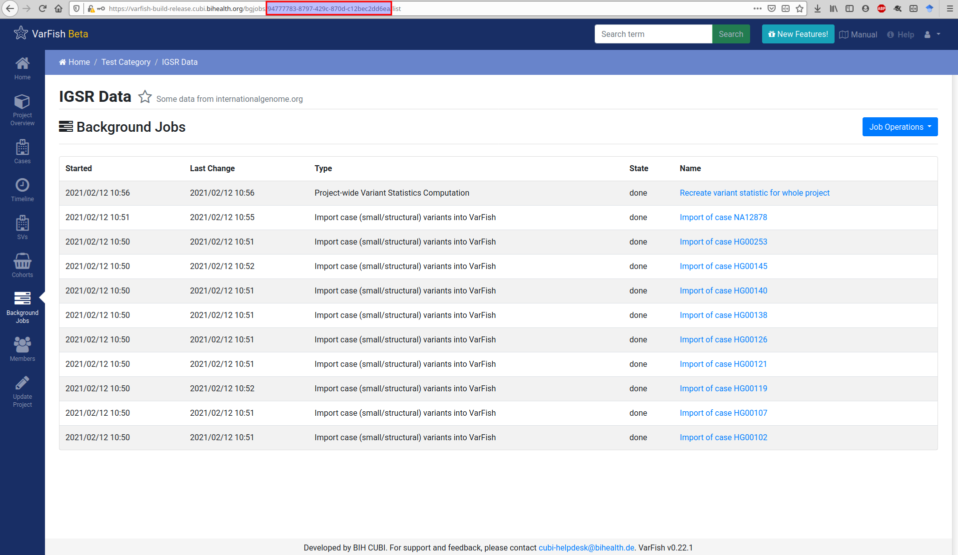
For the import you will also need the project UUID. You can get this from the URLs in VarFish that list project properties. The figure below shows this for the background job list but this also works for the project details view.
$ varfish-cli --no-verify-ssl case create-import-info --resubmit \
    94777783-8797-429c-870d-c12bec2dd6ea \
    test-data/tsv/HG00102-N1-DNA1-WES1/*.{tsv.gz,.ped}
When executing the import as shown above, you have to specify:
a pedigree file with suffix
.ped,a genotype annotation file as generated by
varfish-annotatorending in.gts.tsv.gz,a database info file as generated by
varfish-annotatorending in.db-info.tsv.gz.
Optionally, you can also specify a TSV file with BAM quality control metris ending in .bam-qc.tsv.gz.
Currently, the format is not properly documented yet but documentation and supporting tools are forthcoming.
If you want to import structural variants for your case, then you simply submit the output files from the SV annotation step together with the the .feature-effects.tsv.gz and .gts.tsv.gz files from the small variant annotation step.
Running the import command through VarFish CLI will create a background import job as shown below. Once the job is done, the created or updated case will appear in the case list.
Case Quality Control
You can provide an optional TSV file with case quality control data.
The file name should end in .bam-qc.tsv.gz and also accompanied with a MD5 file.
The format is a bit peculiar and will be documented better in the future.
The TSV file has three columns and starts with the header.
case_id set_id bam_stats
It is then followed by exactly one line where the first two fields have to have the value of a dot (.).
The last row is then a PostgreSQL-encoded JSON dict with the per-sample quality control information.
You can obtain the PostgreSQL-encoding by replacing all string delimiters (") with three ones (""""`).
The format of the JSON file is formally defined in varfish-server case QC info.
Briefly, the keys of the top level dict are the sample names as in the case that you upload. On the second level:
bamstatsThe keys/values from the output of the
samtools statscommand.min_cov_targetCoverage histogram per target (the smallest coverage per target/exon counts for the whole target). You provide the start of each bin, usually starting at
"0", in increments of 10, up to"200". The keys are the bin lower bounds, the values are of JSON/JavaScriptnumbertype, so floating point numbers.min_cov_baseThe same information as
min_cov_targetbut considering coverage base-wise and not target-wise.summaryA summary of the target information.
idxstatsA per-chromosome count of mapped and unmapped reads as returned by the
samtools idxstatscommand.
You can find the example of a real-world JSON QC file below for the first sample.
{
  "index": {
    "bamstats": {
      "raw total sequences": 154189250,
      "filtered sequences": 0,
      "sequences": 154189250,
      "is sorted": 1,
      "1st fragments": 77094625,
      "last fragments": 77094625,
      "reads mapped": 153919815,
      "reads mapped and paired": 153863370,
      "reads unmapped": 269435,
      "reads properly paired": 153071356,
      "reads paired": 154189250,
      "reads duplicated": 7273644,
      "reads MQ0": 2701485,
      "reads QC failed": 0,
      "non-primary alignments": 129724,
      "total length": 19427845500,
      "total first fragment length": 9713922750,
      "total last fragment length": 9713922750,
      "bases mapped": 19393896690,
      "bases mapped (cigar)": 19238950186,
      "bases trimmed": 0,
      "bases duplicated": 916479144,
      "mismatches": 61093079,
      "error rate": 0.003175489,
      "average length": 126,
      "average first fragment length": 126,
      "average last fragment length": 126,
      "maximum length": 126,
      "maximum first fragment length": 126,
      "maximum last fragment length": 126,
      "average quality": 35,
      "insert size average": 192.6,
      "insert size standard deviation": 54.3,
      "inward oriented pairs": 73269191,
      "outward oriented pairs": 3391556,
      "pairs with other orientation": 12579,
      "pairs on different chromosomes": 258359,
      "percentage of properly paired reads (%)": 99.3
    },
    "min_cov_target": {
      "0": 100,
      "10": 87.59,
      "190": 12.31,
      "200": 10.74
    },
    "min_cov_base": {
      "0": 100,
      "10": 95.89,
      "190": 46.55,
      "200": 43.88
    },
    "summary": {
      "mean coverage": 206.69,
      "target count": 232447,
      "total target size": 57464133
    },
    "idxstats": {
      "1": {
        "mapped": 14553406,
        "unmapped": 5166
      },
      "MT": {
        "mapped": 10058,
        "unmapped": 7
      },
      "*": {
        "mapped": 0,
        "unmapped": 212990
      }
    }
  },
  "father": {
    "bamstats": {